Digital Baseband Transmission and Frequency-Domain Analysis
Two MATLAB studies from 2024 that share a subject: what happens to a signal between a source and a decision. The first builds a complete baseband link—source, pulse shaping, an additive noise channel, a matched filter, sampling, a threshold decision—and measures its bit error rate against theory over a million symbols. The second goes underneath it: the discrete Fourier transform and its inverse written from the definition, and what a sampling rate does to a spectrum.
Why build the chain rather than call it
A baseband link can be simulated in a dozen lines by calling a toolbox: one function shapes, one adds noise, one detects, one counts. Every stage of this one is written from primitives instead, and that was the decision the whole study rests on. A toolbox call is correct by assumption; a stage you wrote is correct only if its output agrees with what theory says it should be. Building the chain is what makes the final curve evidence rather than a plot.
It also puts the design decisions where they can be seen. Upsampling factor, filter length, where the convolution transient is trimmed, which sample of each symbol period the detector takes, which side of the threshold a tie falls on—each of those is a choice, and each of them moves the measured curve if it is made wrong. The agreement with theory at the end is a statement that none of them was.
The link, end to end
Every stage is written from primitives rather than assembled out of a toolbox: the line coder and its decoder, the filter that convolves and then trims the transient at both ends, the sampler that takes one value per symbol period, the threshold decision, and the routine that counts disagreements between what went in and what came out.
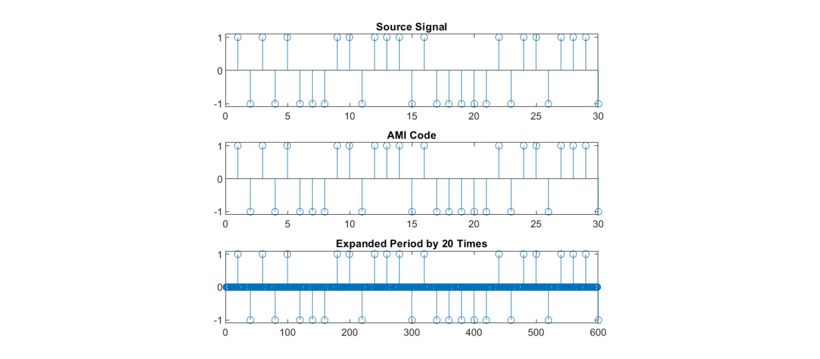
A source of a million symbols is generated, encoded, and stretched by a factor of twenty so each symbol becomes an impulse with nineteen zeros behind it. That upsampled train is what the shaping filter turns into a waveform.
Two pulse shapes
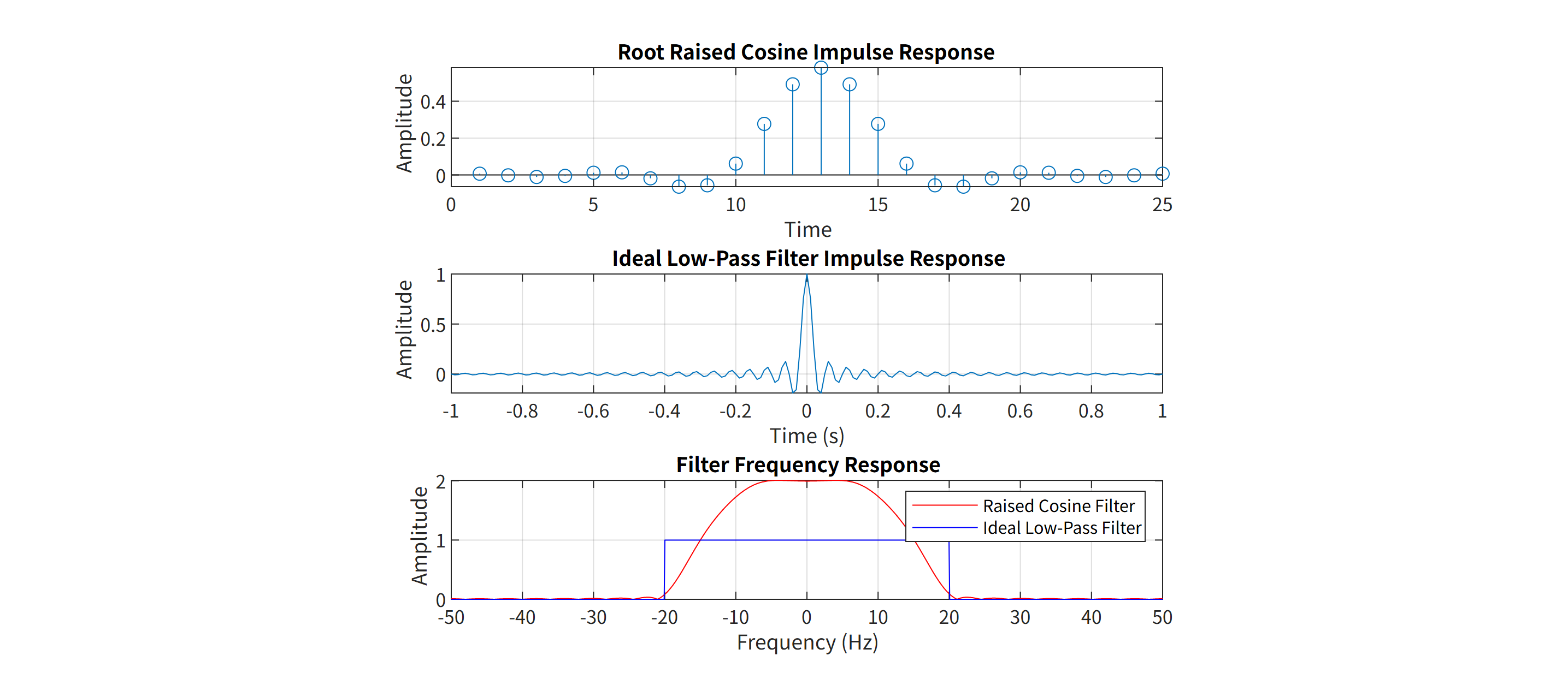
The link is built twice, once with each of two shaping filters, because the comparison is the point of the study. One is the ideal low-pass filter: a rectangle in frequency, which makes it a sinc in time—infinitely long, and ringing on both sides of every symbol. The other is a root raised cosine with a roll-off of 0.6: it gives up part of the bandwidth in exchange for a pulse that decays quickly and crosses zero at every other symbol instant.
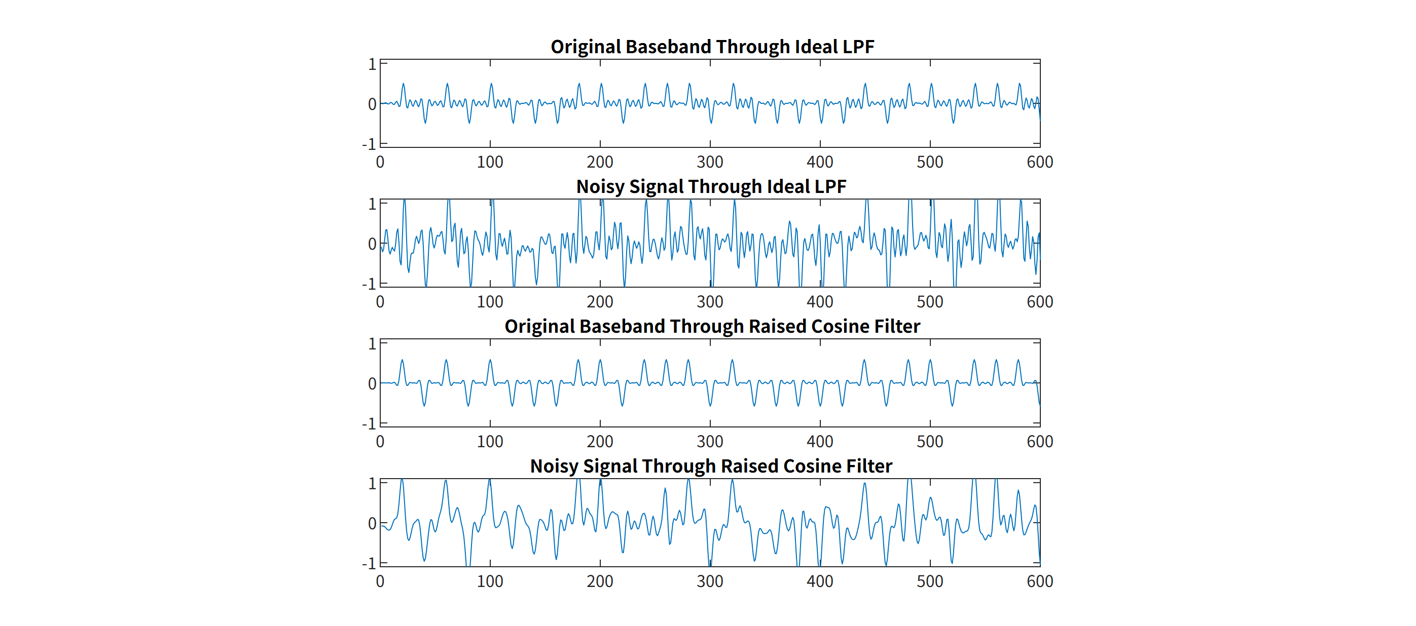
Putting the same source through both, with and without noise, shows what that trade looks like on the wire. Under the ideal filter the waveform carries the tails of neighbouring symbols; under the root raised cosine those tails are gone by the time the next symbol is sampled.
Sampling and the decision
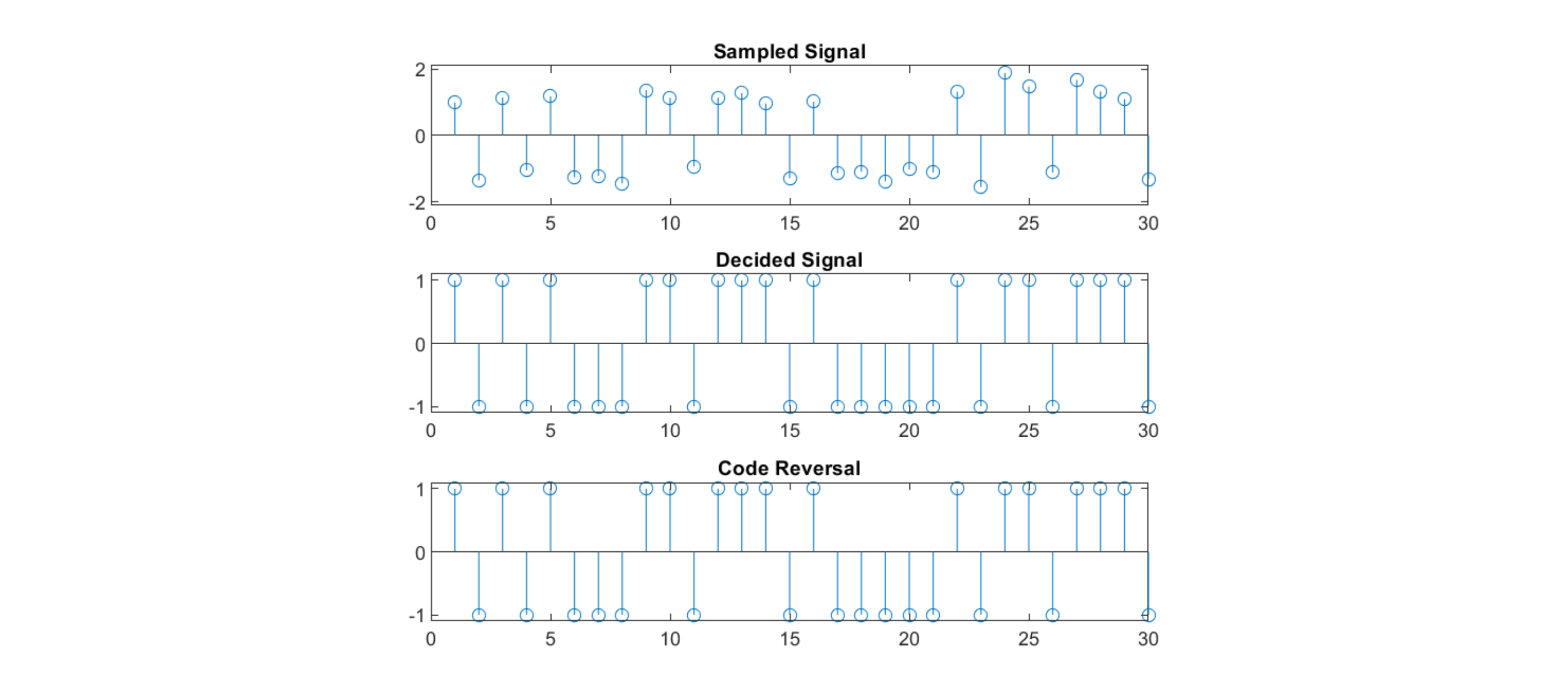
At the receiver the signal goes through the same root raised cosine again. Two of these in series make one raised cosine, which is the shape that is zero at every symbol instant except its own, so the matched filter and the intersymbol-interference condition are satisfied by the same pair of filters. The output is sampled once per symbol period, the sample is compared against a threshold, and the decision is mapped back to a source symbol.
Where in the symbol to take that sample is a design question of its own, and the eye diagram is how it gets settled. Overlaying the received waveform one symbol period at a time collapses the whole stream into a single picture: the vertical opening at the decision instant is the margin the threshold has against noise, and the horizontal opening is how far the sampling instant may drift before intersymbol interference from the neighbouring symbols starts to matter. The two filters separate here as sharply as they do in the waveforms above. The sinc tails of the ideal low-pass filter carry through the decision region and close the eye; the root raised cosine pair, zero at every symbol instant but its own, keeps the crossings bunched and the eye open. I formed the eye for both filters, and used it to place the sampling instant and to read the timing margin the link tolerates.
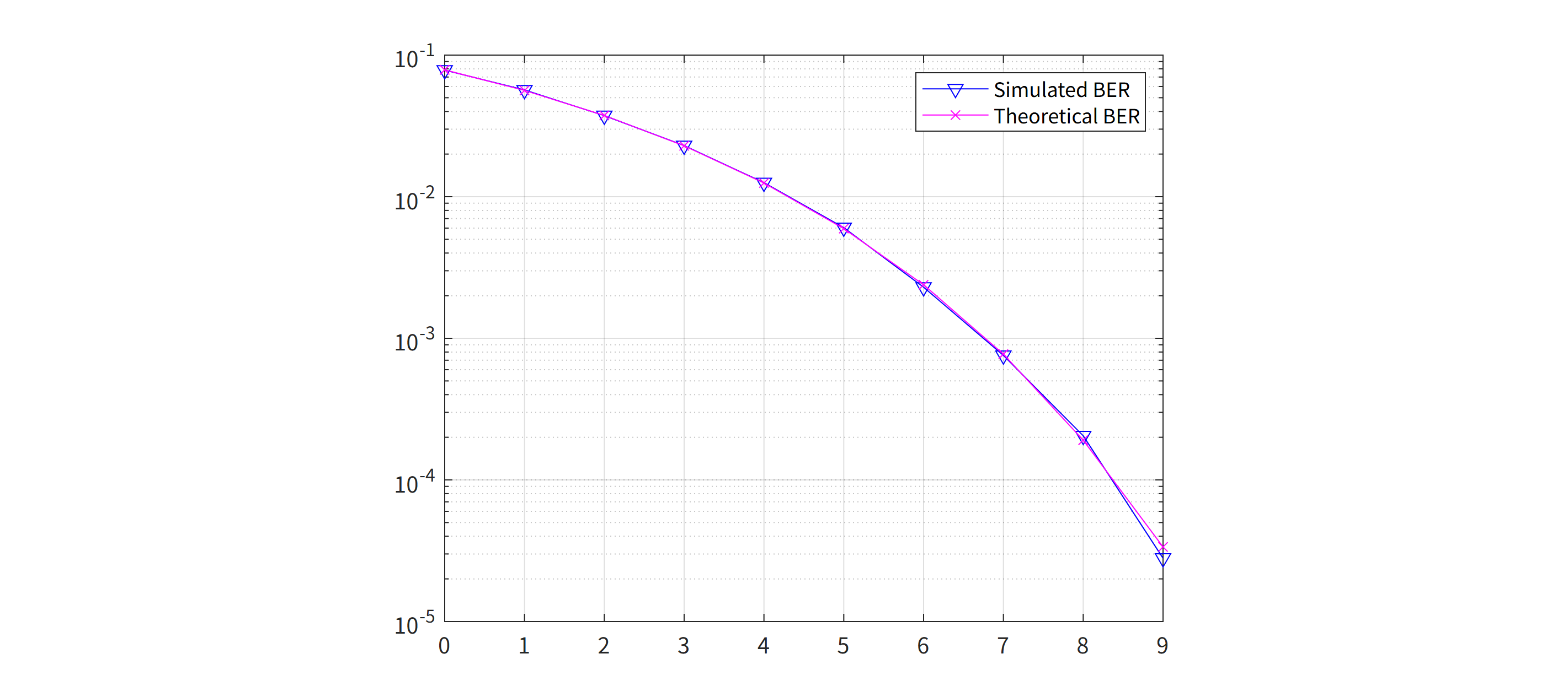
That whole chain is then run ten times, at signal-to-noise ratios from 0 to 9 dB, a million
symbols each, and the measured error rate is plotted against
erfc(√SNR)/2. The two curves lie on top of each other over three decades. That
agreement is the check on the implementation: a wrong filter length, a sampler off by one, or a
threshold on the wrong side would move the measured curve away from the analytic one, and it does
not move.
What the curve settles
Ten operating points, a million symbols each, and the measured error rate lands on
erfc(√SNR)/2 across three decades. That is a stronger check than it looks. The
theoretical expression assumes the detector is matched to the transmit pulse, that the sampling
instant is the one where the combined response peaks, and that the intersymbol contribution at
every other instant is zero. A chain that satisfies all three lies on the curve; a chain that
satisfies none of them can still produce a plausible-looking curve of its own, just displaced. The
distance between measurement and theory is therefore a test of the implementation, and it is the
reason the study runs a million symbols per point rather than a thousand: at the low-error end the
measurement has to resolve a rate near three in a hundred thousand before the comparison means
anything.
Writing the transform
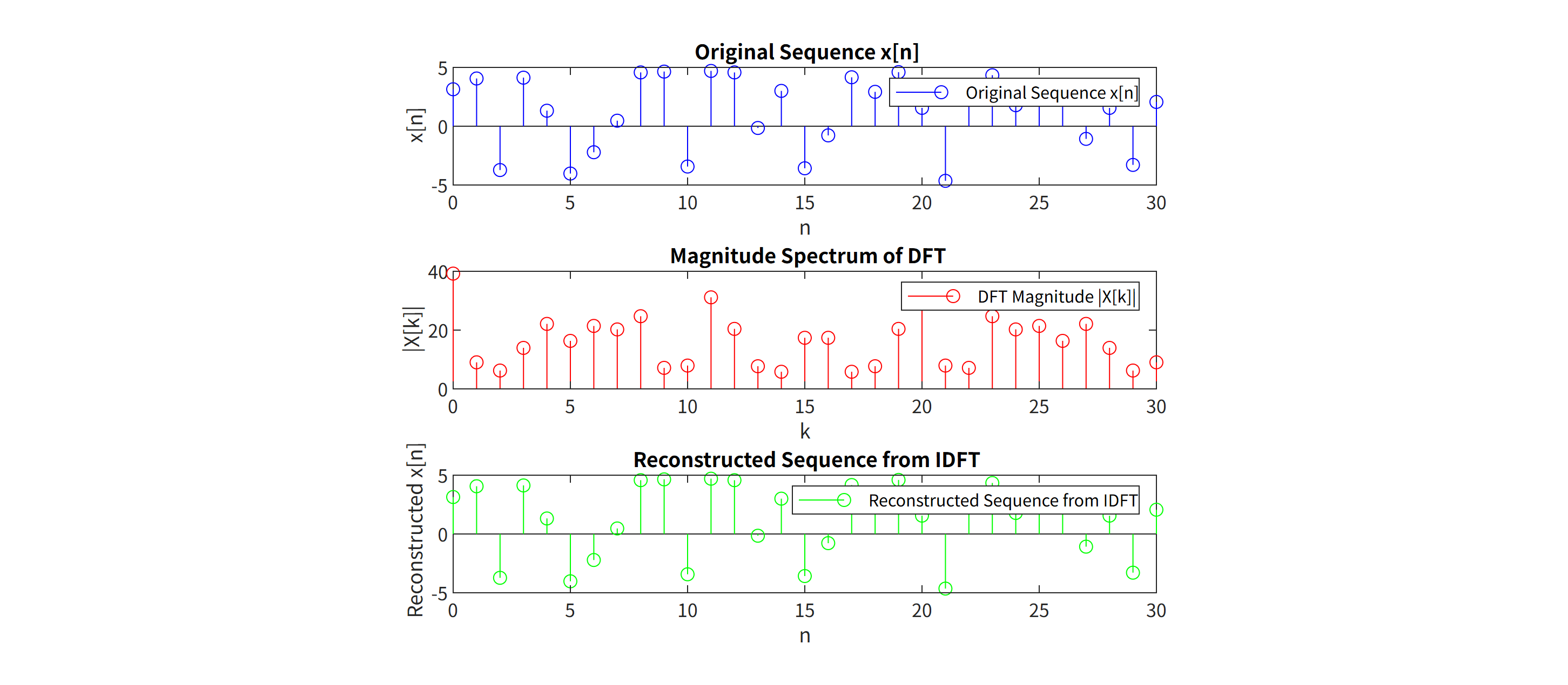
The second study starts one level down, with the transform itself. The DFT is written as its
defining sum over the sequence, the IDFT as the matching sum back, and both are then run against
MATLAB's own fft and ifft on the same input. Reconstructing the sequence
from its own spectrum and getting the original back is what says the pair is right.
What the sampling rate does
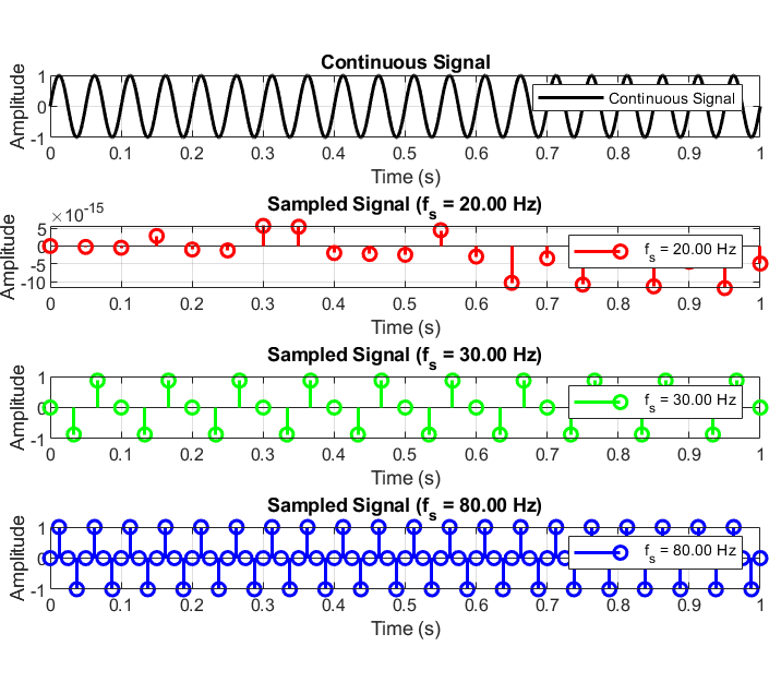
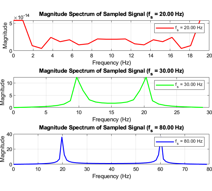
A 20 Hz sinusoid is then sampled at three rates and each result is taken back to the frequency domain. At 80 Hz the rate is above twice the signal frequency and the spectrum shows the tone where it belongs. At 30 Hz it is below, and the tone folds down to 10 Hz—a frequency that was never in the signal. At 20 Hz the rate equals the signal frequency, every sample lands at the same point of the cycle, and the sampled sequence is a constant.