Handwritten Chinese Sentence Recognition Using CNN-CTC

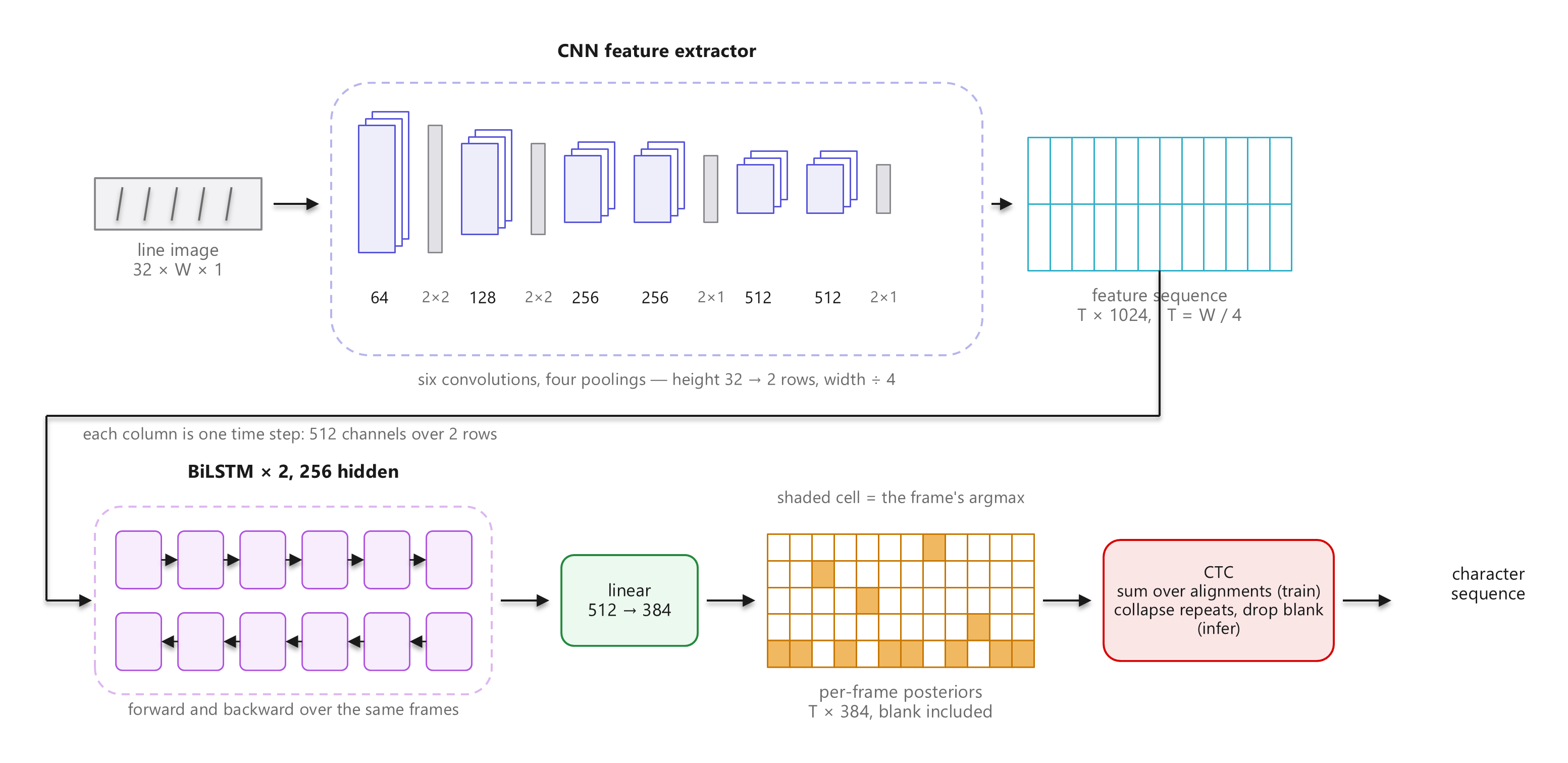
A recognizer for handwritten Chinese written in 2024: a line of handwriting goes in and a string of characters comes out, with nothing in between that has to decide where one character ends and the next begins. A convolutional network reads the line image, two bidirectional LSTM layers read what the convolutions produce, and a CTC head turns a sequence of per-frame predictions into text. The data is CASIA-HWDB, parsed from its own binary formats.

The network drawn as two rows. Top: a 32-pixel-tall line image enters a CNN of four convolution stages, 64 to 512 channels, whose height is pooled to one and whose width is pooled by four, giving a feature sequence of T columns of 512 values. Bottom: that sequence runs through two bidirectional LSTM layers of 256 hidden units in both directions, a linear layer to 384, and a T by 384 matrix of per-frame posteriors that the CTC head turns into a character sequence. — The image is reduced in height until it is a sequence; the sequence is what the recurrent layers and the CTC head work on. Blank is one of the 384 classes, which is what lets a frame decline to emit a character.

Reading a line whole

The direct approach to a line of Chinese is to cut it into characters and classify each one. On handwriting the cut is the hard part: strokes of neighbouring characters run into one another, spacing changes with the writer and with how much room is left at the end of a line, and a cut in the wrong place costs two characters rather than one. Every later stage inherits whatever that step got wrong.

CTC removes the step. The network produces a prediction for every frame of the image; a blank symbol lets a frame say that nothing ends there; and the loss sums over every alignment between the frame sequence and the target string. Training needs only the line and what it says. Where the characters fall is something the model settles for itself.

The alignment nobody labels

What CTC has to reconcile is a mismatch in length. The network emits one distribution per frame, and a 256-pixel line arrives at the head as 64 frames; the label is a string of perhaps a dozen characters. Nothing in the data says which frames belong to which character, and I did not want a system that needed to be told.

The blank symbol is what closes the gap. Any frame may emit blank, meaning “nothing ends here”, so a single label expands into an enormous family of frame sequences: a character may occupy one frame or twenty, and blanks may sit anywhere between. Collapsing runs of the same class and then dropping the blanks maps every member of that family back to the same string. The loss is the total probability of the family—summed over every path, not over one chosen alignment —and it is computed by a forward recursion rather than by enumeration, which is what makes an exponential number of paths a linear amount of work.

Two consequences shape the rest of the design. The frame count has to exceed the label length, or no path exists and the loss is undefined—which is why the pooling is asymmetric, and why the width of the image is protected all the way to the recurrent layers. And the order of the two decoding steps matters: collapsing before dropping blanks is what lets a genuinely doubled character survive, because the blank the network places between the two occurrences is the only thing separating them.

The data

CASIA-HWDB ships in two binary formats, and I wrote a reader for each.

.gnt holds isolated characters. Each record is length-prefixed, carries a GB2312 tag code and then a raw bitmap with its own width and height. The reader walks the file record by record, decodes the tag to a character, keeps it only if it belongs to the vocabulary, caps each class so no character dominates the set, and splits into training and test under a fixed seed so the split is the same every run.

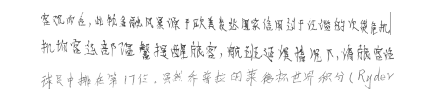
.dgrl holds sentences as pen strokes: a stroke count, then a point list per stroke, then a UTF-16LE label. The reader draws those strokes into a grayscale line image at the height the network expects, scaling the whole line to fit rather than each character, which is what preserves the spacing and slant of one writer across the line.

Three lines of handwritten Chinese text from the CASIA-HWDB sentence data, each rendered as a single wide grayscale image — Three lines rendered from the stroke data. The model sees a whole line at a time, at the width the writer produced.

The vocabulary is a fixed list of 383 characters rather than the full GB2312 set. Holding it fixed sets the output layer at 384 units including the blank, and it keeps the number of samples per class high enough to be worth learning from at this data scale.

The network

Six convolutional layers take the image from one channel to 512, with batch normalization at the two points where the channel count jumps. The pooling is where the design sits. The first two pools halve both dimensions. The last two are 2×1: they halve the height and leave the width untouched. By the end the height has collapsed to 2 rows while the width has only been divided by four.

That asymmetry is the point. Height is what the convolutions are meant to absorb into a feature vector; width is time, and time has to survive. A 256-pixel line arrives at the recurrent layers as 64 frames, comfortably more than the number of characters on it—which is the condition CTC needs, since the frame count has to exceed the label length for an alignment to exist.

The feature map is then reshaped so that each column of the image is one time step carrying 1,024 features, 512 channels over 2 remaining rows. Two bidirectional LSTM layers with 256 hidden units read that sequence in both directions, because what a stroke is often depends on what follows it as much as on what precedes it. A linear layer maps every frame to 384 scores.

Training and decoding

Training uses the CTC loss with the blank at the last index, Adam at 1e-3, batches of 64, and 20 epochs, keeping the checkpoint with the lowest validation loss. Because every image is padded to a common width, the input length is the same for every sample in a batch, and only the target lengths vary.

Decoding is the greedy path: take the highest-scoring class at each frame, collapse runs of the same class, then drop the blanks. Collapsing before dropping is what lets a genuinely repeated character survive—the blank the model puts between the two occurrences is what keeps them apart.